Silver bullet
Adaboost & Gradient Boosting & XGBoost / Gradient Boosting regression & classification 실습 코드 본문
Adaboost & Gradient Boosting & XGBoost / Gradient Boosting regression & classification 실습 코드
밀크쌀과자 2024. 7. 10. 00:431. XGBoost (Extreme Gradient Boosting)
- 대용량 분산 처리를 위한 그래디언트 부스팅 오픈소스 라이브러리
의사결정나무(Decision Tree)에 Boosting 기법을 적용한 알고리즘 (라이브러리)
→ 빠르고 유연한 지도 학습 알고리즘, Kaggle 등에서 우승한 많은 팀들이 선택한 알고리즘으로 주목을 받으며 많은 인기를 얻음

Decision Tree (의사결정나무)
: 이해하기 쉽고 해석도 용이함. 그러나 입력 데이터의 작은 변동에도 Tree의 구성이 크게 달라질 수 있음 & 과적합이 쉽게 발생
성능이 잘 나오지 않음...
→ 이를 해결하기 위해 Boosting 기법이 활용됨 (model ensemble 기법 중 하나)
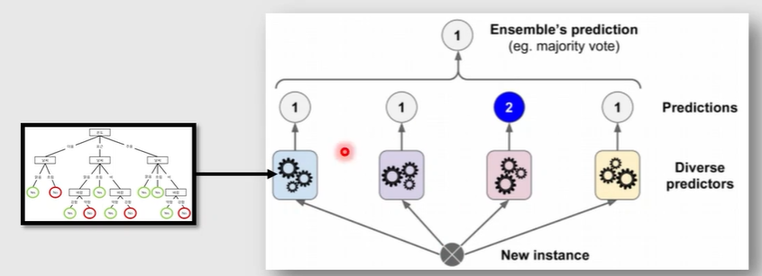
Ensemble
1. Boosting
2. Bagging
Boosted Decision Tree
- Boosting : 'Weak learner'들을 'strong learner'로 변환시키는 알고리즘 = 약한 학습기를 여러개 사용하여 하나의 강건한 학습기를 만들어내는 것

1) Regression : 평균 / 가중평균
2) Classification : 투표
XG Boost
Boosting Algorithm
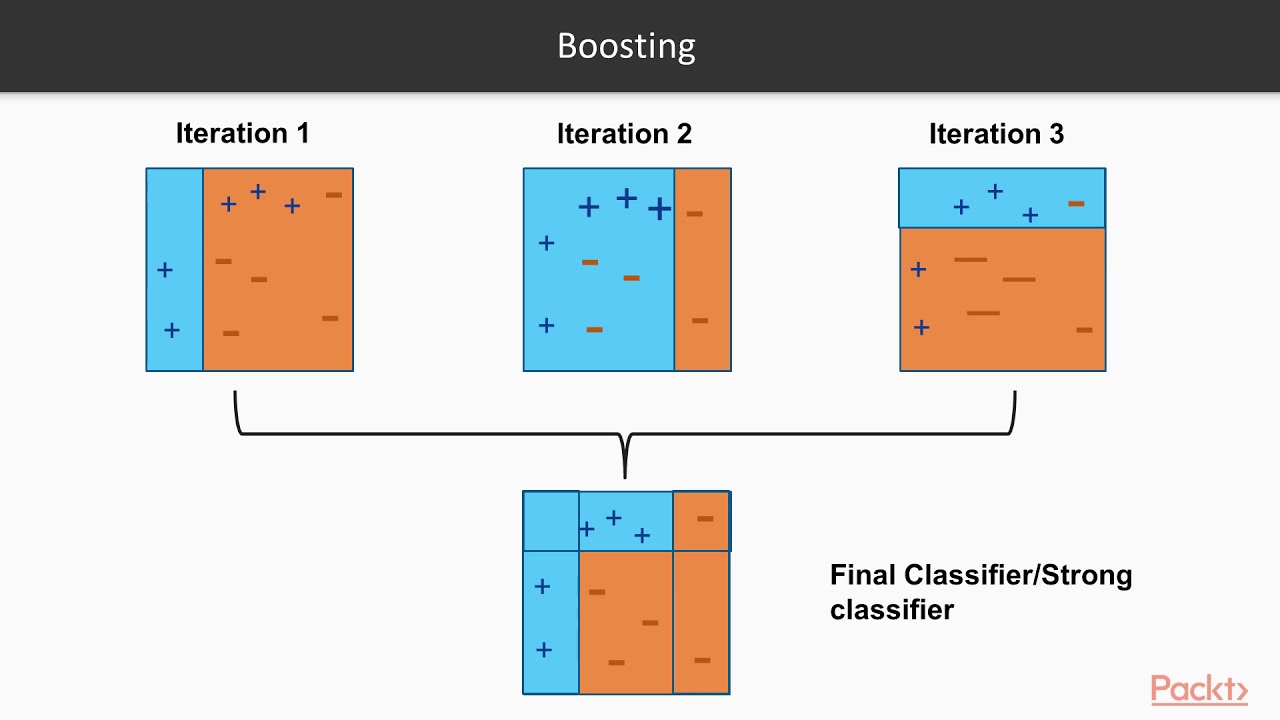
1. AdaBoost (Adaptive Boosting)
- 데이터를 바탕으로 여러 weak learner들을 반복적으로 생성
- 매번 앞선 learner가 잘못 예측한 데이터에 가중치를 부여하고 (boosting) 학습
- 최종적으로 만들어진 strong learner를 이용하여 실제 예측 진행

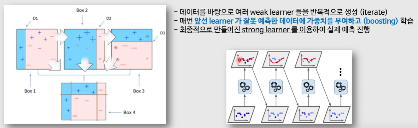
AdaBoost는 높은 weight를 가진 data point가 존재하게 되면 성능이 크게 떨어지는 단점이 있음
(높은 weight를 가진 data point에 가까운 다른 data point들이 잘못 분류될 가능성이 높아짐)
어떻게 하면 에러를 최소화하는 방향으로 weight를 매겨줄 수 있을까?
→ Gradient Boosting (2012) : 경사하강법을 사용해서 AdaBoost보다 성능을 개선한 Boosting 기법 / Gradient descent를 적용하여 가중치들에 대한 update를 진행
Boosting Algorithm
2. Gradient Boosting
: 경사 하강법을 사용하여 AdaBoost보다 성능을 개선한 Boosting 기법
→ 학습 성능은 좋으나, 모델의 학습 시간이 오래 걸리는 단점이 발생
→ XG Boost (Extreme Gradient Boosting, 2016) : 병렬 처리 기법을 적용하여 Gradient Boost보다 학습 속도를 크게 끌어올림 (구체적으로는 Tree를 구성할 때, 각 Tree의 노드는 어떤 feature로 가지를 쳐야할지 결정하는 과정 중 예측값 계산에 병렬처리를 사용)
Boosting Algorithm
3. XG Boosting
: 병렬 처리 기법 → 시간 효율성 증가
하이퍼파라미터가 많음 (3~40개)
sklearn에는 없고, 별도로 설치해서 써야함
→ Light GBM (2018) : MS사에서 개발
Gradient Boosting regression 실습
https://scikit-learn.org/0.20/auto_examples/ensemble/plot_gradient_boosting_regression.html
import numpy as np
import matplotlib.pyplot as plt

from sklearn import ensemble
from sklearn import datasets
from sklearn.utils import shuffle
from sklearn.metrics import mean_squared_error

# Load data
# train_test_split을 손으로 하는 코드
boston = datasets.load_boston()
X, y = shuffle(boston.data, boston.target, random_state=13)

X = X.astype(np.float32)
offset = int(X.shape[0] * 0.9)

X_train, y_train = X[:offset], y[:offset]
X_test, y_test = X[offset:], y[offset:]
# Fit regression model
params = {'n_estimators': 500, 'max_depth': 4, 'min_samples_split': 2,
'learning_rate': 0.01, 'loss': 'ls'}
clf = ensemble.GradientBoostingRegressor(**params)
clf = ensemble.GradientBoostingRegressor(n_estimators=500,
max_depth=4,
min_samples_split=2,
learning_rate=0.01,
loss='ls')
clf.fit(X_train, y_train)
mse = mean_squared_error(y_test, clf.predict(X_test))
print("MSE: %.4f" % mse)MSE: 6.7659n_estimators : 의사결정나무 개
max_dapth : 의사 결정 나무 깊이 설정
min_samples_split : 최소로 나눠졌을때 제한 개수
loss : ls(least Squares estimation) → MSE와 비슷
clf → classifier
reg → regression
# compute test set deviance
# 회귀 분석에서만 돌아가는 코드
test_score = np.zeros((params['n_estimators'],), dtype=np.float64)

for i, y_pred in enumerate(clf.staged_predict(X_test)):
    test_score[i] = clf.loss_(y_test, y_pred)

plt.figure(figsize=(12, 6))
plt.subplot(1, 2, 1)
plt.title('Deviance')
plt.plot(np.arange(params['n_estimators']) + 1, clf.train_score_, 'b-',
         label='Training Set Deviance')
plt.plot(np.arange(params['n_estimators']) + 1, test_score, 'r-',
         label='Test Set Deviance')
plt.legend(loc='upper right')
plt.xlabel('Boosting Iterations')
plt.ylabel('Deviance') #에러
clf.staged_predict : 의사결정나무 만들때 마다 predict한 결과
clf.feature_importances_# Plot feature importance
# Plot feature importance
feature_importance = clf.feature_importances_

# make importances relative to max importance
feature_importance = 100.0 * (feature_importance / feature_importance.max())
sorted_idx = np.argsort(feature_importance)
pos = np.arange(sorted_idx.shape[0]) + .5

plt.figure(figsize=(10, 5))
plt.subplot(1, 2, 2)
plt.barh(pos, feature_importance[sorted_idx], align='center')
plt.yticks(pos, boston.feature_names[sorted_idx])
plt.xlabel('Relative Importance')
plt.title('Variable Importance')
plt.show()
Gradient Boosting regression (diabetes dataset) 실습
https://scikit-learn.org/stable/auto_examples/ensemble/plot_gradient_boosting_regression.html
import matplotlib.pyplot as plt
import numpy as np
from sklearn import datasets, ensemble
from sklearn.metrics import mean_squared_error
from sklearn.model_selection import train_test_split

from sklearn.inspection import permutation_importance

diabetes = datasets.load_diabetes()
X, y = diabetes.data, diabetes.target

print(diabetes['DESCR'])

X_train, X_test, y_train, y_test = train_test_split(
    X, y, test_size=0.1, random_state=13)

params = {'n_estimators': 2000,
          'max_depth': 4,
          'min_samples_split': 5,
          'learning_rate': 0.01,
          'loss': 'ls'}

# "ls" 관련 에러 발생 시 "ls"를 "squared_error"로 수정해주세요!

reg = ensemble.GradientBoostingRegressor(**params)
reg.fit(X_train, y_train)

mse = mean_squared_error(y_test, reg.predict(X_test))
print("The mean squared error (MSE) on test set: {:.4f}".format(mse))
test_score = np.zeros((params['n_estimators'],), dtype=np.float64)
for i, y_pred in enumerate(reg.staged_predict(X_test)):
test_score[i] = reg.loss_(y_test, y_pred)
fig = plt.figure(figsize=(6, 6))
plt.subplot(1, 1, 1)
plt.title('Deviance')
plt.plot(np.arange(params['n_estimators']) + 1, reg.train_score_, 'b-',
label='Training Set Deviance')
plt.plot(np.arange(params['n_estimators']) + 1, test_score, 'r-',
label='Test Set Deviance')
plt.legend(loc='upper right')
plt.xlabel('Boosting Iterations')
plt.ylabel('Deviance')
fig.tight_layout()
plt.show()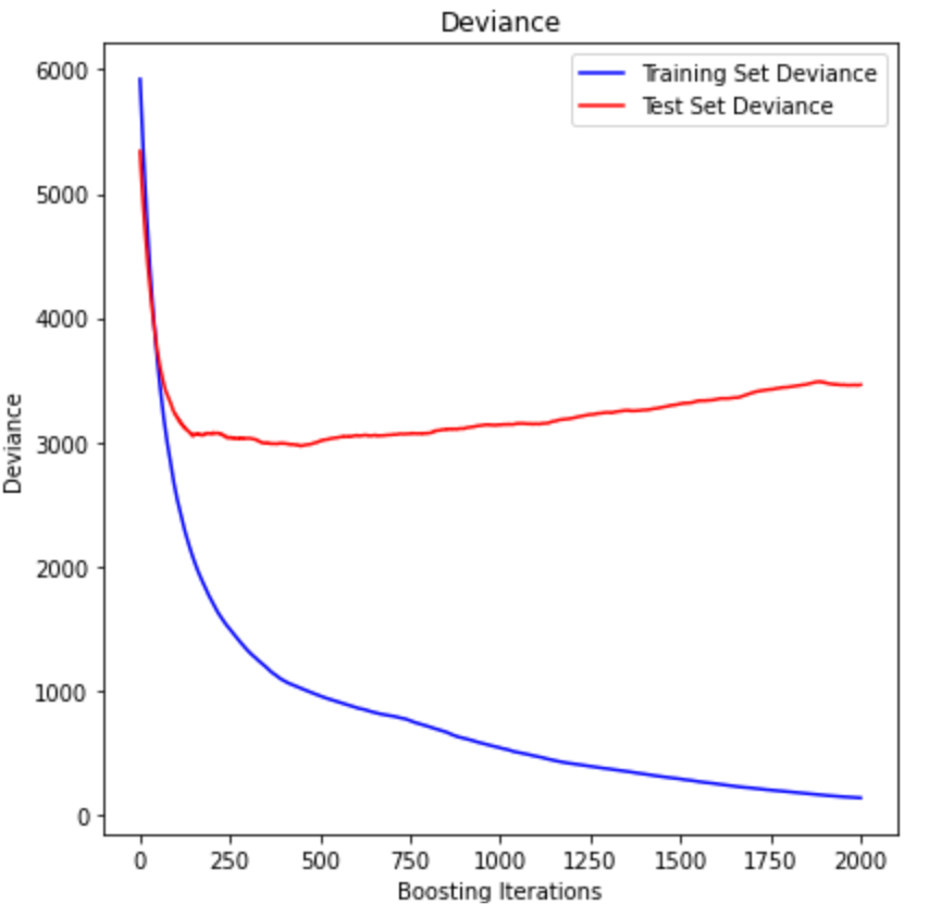
reg.feature_importances_

feature_importance = reg.feature_importances_

sorted_idx = np.argsort(feature_importance)
pos = np.arange(sorted_idx.shape[0]) + .5

fig = plt.figure(figsize=(12, 6))
# plt.subplot(1, 2, 1)

plt.barh(pos, feature_importance[sorted_idx], align='center')
plt.yticks(pos, np.array(diabetes.feature_names)[sorted_idx])
plt.title('Feature Importance (MDI)')

# result = permutation_importance(reg, X_test, y_test, n_repeats=10, random_state=42, n_jobs=2)
# sorted_idx = result.importances_mean.argsort()
# plt.subplot(1, 2, 2)
# plt.boxplot(result.importances[sorted_idx].T, vert=False, labels=np.array(diabetes.feature_names)[sorted_idx])
# plt.title("Permutation Importance (test set)")

fig.tight_layout()
plt.show()
fig = plt.figure(figsize=(12, 6))
result = permutation_importance(reg, X_test, y_test, n_repeats=10, random_state=42, n_jobs=2)
sorted_idx = result.importances_mean.argsort()
plt.boxplot(result.importances[sorted_idx].T, vert=False, labels=np.array(diabetes.feature_names)[sorted_idx])
plt.title("Permutation Importance (test set)")
fig.tight_layout()
plt.show()Permutation Importance가 Feature Importance보다 신뢰도가 좀 더 높다. (Permutation Importance를 그려내지 못하는 모델도 있음)
result = permutation_importance(reg, X_test, y_test, n_repeats=10, random_state=42, n_jobs=2)
n_repeats : 값을 섞는 횟수 (K-Fold와 비슷한 느낌)
n_jobs : 병렬 프로그래밍
Permutation Importance
: 모델에 대하여 특정 Feature를 안 썼을 때, 이것이 성능 손실에 얼마만큼의 영향을 주는지를 통해 그 feature의 중요도를 파악하는 방법
Permutation Importance 특징
: 재학습 시킬 필요가 없다. 변수를 아예 포함하지 않는 것 대신, 그 feature의 값들을 무작위로 섞어서(permutation) 그 feature를 노이즈로 만드는 것입니다.! 무작위로 섞게 되면, 목표 변수와 어떠한 연결고리를 끊게 되는 것이므로, 그 feature를 안 쓴다고 할 수 있을 것입니다. 이렇게 섞었을 때 예측값이 실제 값보다 얼마나 차이가 더 생겼는지를 통해 해당 feature의 영향력을 파악합니다.
import pandas as pd

pd.DataFrame(result.importances) # 행방향 : x데이터 기준, 열방향 : 우리가 설정한 10번의 시도
result['importances'].mean(axis=1)
result['importances_mean']
reg.score(X_test, y_test)
- Regression -> model.score(x, y) == R2 score (1에 가까울수록 모델의 설명력이 좋음 vs 0에 가까울수록 모델의 설명력이 떨어짐)
- Classification -> model.score(x, y) == Accuracy score (1에 가까울수록 모델이 분류를 정확하게 해냄)- Regression -> model.score(x, y) == R2 score
- Classification -> model.score(x, y) == Accuracy score
Gradient Boosting classification (breast-cancer dataset)
import numpy as np
import pandas as pd
import matplotlib.pyplot as plt

from sklearn import datasets, ensemble
from sklearn.metrics import accuracy_score
from sklearn.model_selection import train_test_split

cancer = datasets.load_breast_cancer()
X, y = cancer.data, cancer.target

X_train, X_test, y_train, y_test = train_test_split(
    X, y, test_size=0.1, random_state=13)

params = {'n_estimators': 1000,
          'max_depth': 4,
          'min_samples_split': 5,
          'learning_rate': 0.01}

          clf = ensemble.GradientBoostingClassifier(**params)
clf.fit(X_train, y_train)

acc = accuracy_score(y_test, clf.predict(X_test))
print("The accuracy score on test set: {:.4f}".format(acc))
The accuracy score on test set: 0.9123clf.score(X_test, y_test)0.9122807017543859classification의 score은 accuracy이므로 같은 값이 나온다.
import pandas as pd

pd.DataFrame(cancer.target)[0].value_counts()

train_score = np.zeros((params['n_estimators'],), dtype=np.float64)
for i, y_pred in enumerate(clf.staged_predict(X_train)):
    train_score[i] = accuracy_score(y_train, y_pred)

test_score = np.zeros((params['n_estimators'],), dtype=np.float64)
for i, y_pred in enumerate(clf.staged_predict(X_test)):
    test_score[i] = accuracy_score(y_test, y_pred)

fig = plt.figure(figsize=(12, 6))
plt.subplot(1, 1, 1)
plt.title('Accuracy') # Binomial deviance loss function for binary classification
plt.plot(np.arange(params['n_estimators']) + 1, train_score, 'b-', label='Training Set Accuracy')
plt.plot(np.arange(params['n_estimators']) + 1, test_score, 'r-', label='Test Set Accuracy')
plt.legend(loc='upper right')
plt.xlabel('Boosting Iterations')
plt.ylabel('Accuracy')
fig.tight_layout()
plt.show()
feature_importance = clf.feature_importances_
sorted_idx = np.argsort(feature_importance)
pos = np.arange(sorted_idx.shape[0]) + .5
fig = plt.figure(figsize=(12, 6))
plt.barh(pos, feature_importance[sorted_idx], align='center')
plt.yticks(pos, np.array(cancer.feature_names)[sorted_idx])
plt.title('Feature Importance (MDI)')
fig.tight_layout()
plt.show()from sklearn.metrics import roc_curve, auc
fpr, tpr, _ = roc_curve(y_true=y_test, y_score=clf.predict_proba(X_test)[:,1]) # real y & predicted y (based on "Sepal width")
roc_auc = auc(fpr, tpr) # AUC 면적의 값 (수치)
plt.figure(figsize=(10, 10))
plt.plot(fpr, tpr, color='darkorange', lw=2, label='ROC curve (area = %0.2f)' % roc_auc)
plt.plot([0, 1], [0, 1], color='navy', lw=2, linestyle='--')
plt.xlim([0.0, 1.0])
plt.ylim([0.0, 1.05])
plt.xlabel('False Positive Rate')
plt.ylabel('True Positive Rate')
plt.legend(loc="lower right")
plt.title("ROC curve")
plt.show()from sklearn.metrics import classification_report
predictions = clf.predict(X_test)
print(classification_report(y_test, predictions)) # Precision, Recall, F1-score 등을 확인할 수 있습니다.
print("Accuracy on Training set: {:.3f}".format(clf.score(X_train, y_train)))
print("Accuracy on Test set: {:.3f}".format(clf.score(X_test, y_test))) precision recall f1-score support
0 0.84 0.89 0.86 18
1 0.95 0.92 0.94 39
accuracy 0.91 57
macro avg 0.89 0.91 0.90 57
weighted avg 0.91 0.91 0.91 57
Accuracy on Training set: 1.000
Accuracy on Test set: 0.912support : 데이터 개수(출현 빈도)
'AI > AI' 카테고리의 다른 글
| K-Nearest Neighbor Algorithm (0) | 2024.07.11 |
|---|---|
| SVM - Soft-margin Kernelized SVM / StandardScaler, HPO & GridSearchCV (0) | 2024.07.10 |
| 로지스틱 회귀 (sigmoid function & Cutoff, Cross-entropy & Softmax, Accuracy & Recall & Precision, ROC Curve & AUC) (0) | 2024.07.09 |
| 선형 회귀 실습(Scikit-learn & One-hot encoding) (0) | 2024.07.08 |
| 비용함수와 경사하강법 (Cost function & MSE) (0) | 2024.07.08 |

