Tensorflow (version 2 code) Mnist / Batch-Normalization 적용

MNIST Batch-Normalization 적용 실습 코드

import tensorflow as tf
from tensorflow.keras import datasets, utils
from tensorflow.keras import models, layers, activations, initializers, losses, optimizers, metrics

import os
os.environ['TF_CPP_MIN_LOG_LEVEL'] = '2' # https://stackoverflow.com/questions/35911252/disable-tensorflow-debugging-information

1. Prepare train & test data (MNIST)

(train_data, train_label), (test_data, test_label) = datasets.mnist.load_data()

train_data = train_data.reshape(60000, 784) / 255.0
test_data = test_data.reshape(10000, 784) / 255.0

train_label = utils.to_categorical(train_label) # 0~9 -> one-hot vector
test_label = utils.to_categorical(test_label) # 0~9 -> one-hot vector

2. Build the model & Set the criterion

model = models.Sequential() 

model.add(layers.Dense(input_dim=28*28, units=256, activation=None, kernel_initializer=initializers.he_uniform())) 
model.add(layers.BatchNormalization())
model.add(layers.Activation('relu')) # layers.ELU or layers.LeakyReLU
model.add(layers.Dropout(rate=0.2))

model.add(layers.Dense(units=256, activation=None, kernel_initializer=initializers.he_uniform())) 
model.add(layers.BatchNormalization())
model.add(layers.Activation('relu')) # layers.ELU or layers.LeakyReLU
model.add(layers.Dropout(rate=0.2))

model.add(layers.Dense(units=10, activation='softmax')) # 0~9 

model.compile(optimizer=optimizers.Adam(), # learning rate 지정 가능
              loss=losses.categorical_crossentropy, 
              metrics=[metrics.categorical_accuracy]) # Precision / Recall / F1-Score 적용하기 @ https://j.mp/3cf3lbi

# metrics.top_k_categorical_accuracy 도 사용가능 -> 매우 많은 클래스를 분류하는 모델일때 사용

# model.compile(optimizer='adam', 
#               loss=losses.categorical_crossentropy, 
#               metrics=['accuracy'])

model.summary()

* metrics = [metrics.top_k_categorical_accuracy] : 예측한 결과값 중 top k중에 실제 정답이 있다면 맞춘걸로 간주하자. → 맞춰야 하는 class가 1000~2000개 정도될 때 사용

3. Train the model

# Training 과정에서 epoch마다 활용할 validation set을 나눠줄 수 있습니다.

history = model.fit(train_data, train_label, batch_size=100, epochs=15, validation_split=0.2)

epoch 시작 시점에

60000행

20% == 12000행

80% == 48000행 -> 100행씩 쪼개면 총 480 batches

4. Test the model

result = model.evaluate(test_data, test_label, batch_size=100)

print('loss (cross-entropy) :', result[0])
print('test accuracy :', result[1])

100/100 [==============================] - 0s 2ms/step - loss: 0.0639 - categorical_accuracy: 0.9822
loss (cross-entropy) : 0.06393961608409882
test accuracy : 0.982200026512146

5. Visualize the result

history.history

history.history.keys()

val_acc = history.history['val_categorical_accuracy']
acc = history.history['categorical_accuracy']

import numpy as np
import matplotlib.pyplot as plt

x_len = np.arange(len(acc))
plt.plot(x_len, acc, marker='.', c='blue', label="Train-set Acc.")
plt.plot(x_len, val_acc, marker='.', c='red', label="Validation-set Acc.")

plt.legend(loc='lower right')
plt.grid()
plt.xlabel('epoch')
plt.ylabel('Accuracy')
plt.show()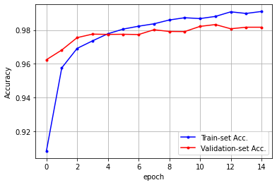

overfitting이 발생했다고 말할 수 없음

val_acc = history.history['val_loss']
acc = history.history['loss']

import numpy as np
import matplotlib.pyplot as plt

x_len = np.arange(len(acc))
plt.plot(x_len, acc, marker='.', c='blue', label="Train-set Acc.")
plt.plot(x_len, val_acc, marker='.', c='red', label="Validation-set Acc.")

plt.legend(loc='upper right')
plt.grid()
plt.xlabel('epoch')
plt.ylabel('Accuracy')
plt.show()