TensorFlow & Linear Regression (version 1 code)

TensorFlow basic

TensorFlow는 1) Building a TensorFlow Graph, 2) Executing the TensorFlow Graph 두 단계를 통해 계산을 수행함

 

Two Steps to perform a computation in TF

1) Building a TensorFlow Graph : Tensor들 사이의 연산 관계를 계산 그래프로 정의 & 선언 == function definition

2) Executing the TensorFlow Graph : 계산 그래프에 정의된 연산(계산)을 tf.Session을 통해 실제로 실행 == function execution

 

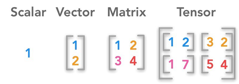
Tensor & Graph

- TensorFlow의 기본 자료 구조 & 타입을 가진 다차원 배열 (본디 "벡터의 확장 개념")

- N-dimensional Matrix

 

---

Tensor basic -- version 1 code --

# tensorflow 버전 1 코드
import tensorflow.compat.v1 as tf
tf.disable_v2_behavior()

import numpy as np
import pandas as pd

a = tf.add(3, 5) # define
print(a)

sess = tf.Session() # 세션을 열고 실행 -> 닫기
print(sess.run(a))
sess.close()

with tf.Session() as sess: # with을 쓰면 close를 쓰지 않아도 된다.
    print(sess.run(a))

x = 2
y = 3
op1 = tf.add(x, y)
op2 = tf.multiply(x, y)
op3 = tf.pow(op2, op1)

with tf.Session() as sess:
    print(type(op3))
    op3 = sess.run(op3)
    print(type(op3))
    print(op3)

<class 'tensorflow.python.framework.ops.Tensor'>
<class 'numpy.int32'>
7776

x = 2
y = 3
op1 = tf.add(x, y)
op2 = tf.multiply(x, y)
useless = tf.multiply(x, op1)
op3 = tf.pow(op2, op1)

with tf.Session() as sess:
    op3, useless = sess.run([op3, useless])
    print(op3, useless)

7776 10

---

Tensor Linear Regression -- version 1 code --

import tensorflow.compat.v1 as tf
tf.disable_v2_behavior()

import numpy as np
import pandas as pd
import matplotlib.pyplot as plt
from sklearn import datasets

x_data = datasets.load_boston().data[:,12]
y_data = datasets.load_boston().target
df = pd.DataFrame([x_data, y_data]).transpose()
df

for name in dir(tf.train):
    if 'Optimizer' in name:
        print(name)
        
w = tf.Variable(tf.random_normal([1])) # 세타 만들기 / 정규분포로부터 랜덤하게 가져오기
b = tf.Variable(tf.random_normal([1]))

y_predicted = w * x_data + b

loss = tf.reduce_mean(tf.square(y_predicted - y_data)) # MSE 만들기
optimizer = tf.train.GradientDescentOptimizer(0.001) # 바닐라 GradientDescent 학습률 지정
train = optimizer.minimize(loss)

with tf.Session() as sess:
    sess.run(tf.global_variables_initializer()) # 세타 초기화
    
    for step in range(10000): # epoch
        sess.run(train) # 실제로 Gradient Descent가 실행되는 코드
        if step % 1000 == 0:
            print(f'Step {step} : w {sess.run(w)} b {sess.run(b)}')
            print(f'loss {sess.run(loss)}')
            print()
    w_out, b_out = sess.run([w, b])

Step 0 : w [0.3020291] b [1.0989273]
loss 428.4620666503906

Step 1000 : w [0.29012078] b [13.897154]
loss 141.4076385498047

Step 2000 : w [-0.18327062] b [21.782118]
loss 77.82865905761719

Step 3000 : w [-0.47596064] b [26.65726]
loss 53.52394485473633

Step 4000 : w [-0.656928] b [29.671515]
loss 44.23274612426758

Step 5000 : w [-0.76881623] b [31.535162]
loss 40.68098831176758

Step 6000 : w [-0.8379954] b [32.68743]
loss 39.32322311401367

Step 7000 : w [-0.88076735] b [33.399857]
loss 38.80418395996094

Step 8000 : w [-0.9072136] b [33.840355]
loss 38.60575866699219

Step 9000 : w [-0.92356443] b [34.1127]
loss 38.5299072265625

plt.figure(figsize=(10, 10))
plt.plot(x_data, y_data, 'bo', label='Real data')
plt.plot(x_data, x_data * w_out + b_out, 'ro', label='Prediction')
plt.legend()
plt.show()

 

---

2-Layer Neural-Network

sigmoid, GradientDescentOptimizer

x_data = datasets.load_boston().data[:,12]
y_data = datasets.load_boston().target
df = pd.DataFrame([x_data, y_data]).transpose()
df

_x_data = tf.reshape(x_data, [len(x_data), 1])
W = tf.Variable(tf.random_normal([1, 5], dtype=tf.float64)) # hidden layer 만들기
W_out = tf.Variable(tf.random_normal([5, 1], dtype=tf.float64))

hidden = tf.nn.sigmoid(tf.matmul(_x_data, W)) # 행렬곱과 sigmod 힘수 씌우기
output = tf.matmul(hidden, W_out) # Regression

loss = tf.reduce_mean(tf.square(output - y_data)) # MSE 만들기
optimizer = tf.train.GradientDescentOptimizer(0.001) # 바닐라 GradientDescent 학습률 지정
train = optimizer.minimize(loss)

with tf.Session() as sess:
    sess.run(tf.global_variables_initializer())
    
    for step in range(50000): # epoch
        sess.run(train)
        if step % 5000 == 0:
            print(f'Step {step} || Loss : {sess.run(loss)}')
            
    output = sess.run(output)
    
plt.figure(figsize=(10, 10))
plt.plot(x_data, y_data, 'bo', label='Real data')
plt.plot(x_data, output, 'ro', label='Prediction')
plt.legend()
plt.show()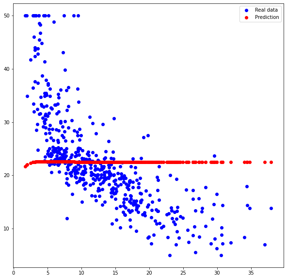

 

why ??? → 함정 : loss = tf.reduce_mean(tf.square(output - y_data)) 부분이다. 

output : (506, 1) / y_data : (506,)

* (중요) y_data도 2차원 행렬이여야 한다.

---

2-Layer Neural-Network

elu, AdamOptimizer

* 변경사항

_y_data = tf.reshape(y_data, [len(y_data), 1]) # [506, 1]

 

loss = tf.losses.mean_squared_error(output, _y_data)

 

_x_data = tf.reshape(x_data, [len(x_data), 1]) # [506, 1]
_y_data = tf.reshape(y_data, [len(y_data), 1]) # [506, 1]

W1 = tf.Variable(tf.random_normal([1, 5], dtype=tf.float64)) # hidden layer 만들기
W2 = tf.Variable(tf.random_normal([5, 10], dtype=tf.float64)) # hidden layer 만들기
W_out = tf.Variable(tf.random_normal([10, 1], dtype=tf.float64))

hidden1 = tf.nn.elu(tf.matmul(_x_data, W1)) # [506, 5]
hidden2 = tf.nn.elu(tf.matmul(hidden1, W2)) # [506, 10]
output = tf.matmul(hidden2, W_out) # [506, 1]

#loss = tf.reduce_mean(tf.square(output - y_data)) # MSE 만들기
loss = tf.losses.mean_squared_error(output, _y_data)
optimizer = tf.train.AdamOptimizer(0.001) # 바닐라 GradientDescent 학습률 지정
train = optimizer.minimize(loss)

with tf.Session() as sess:
    sess.run(tf.global_variables_initializer())
    
    for step in range(50000): # epoch
        sess.run(train)
        if step % 5000 == 0:
            print(f'Step {step} || Loss : {sess.run(loss)}')
            
    output = sess.run(output)
    
plt.figure(figsize=(10, 10))
plt.plot(x_data, y_data, 'bo', label='Real data')
plt.plot(x_data, output, 'ro', label='Prediction')
plt.legend()
plt.show()